April 2019 – fivetwentyone

I’ve recently been working on some code for baseball simulations (in scala, rust, and D – but that’s a whole other blog post). The simulations follow what I’d say is the standard procedure, i.e.

initialize a game state
simulate a batting event
update the state
repeat until the end state

While working on these simulations, it suddenly occurred to me that in order to simulate runs scored, you don’t actually have to simulate a sequence of events, as they might happen in a real game. In fact, the number of runs in an inning is totally specified by

The total number of PA
The number of runners left on base

So instead of simulating events, tracking the evolution of the game state, and keeping a running total of runs scored, we can compute $P(L, N)$ , the probability for a given set of PA ( $N$ ) and runners left on base ( $L$ ), and $R(L, N)$ , the runs scored, as a function of PA and left-on-base. A given sequence of events determines the number of runners left on base, so we can write more specifically,

$P(L, N) = P(S|C) P(C|N) P(N)$ ,

where $S$ represents a sequence, $C$ represents a combination and $N$ is the number of total PA. As an example in the sequence BB – HR – BB, the combination, $C$ , is (BB=2, HR=1), $N=6$ , $L= 1$ , $R = 2$ . Note also that the number of runners left on base in an inning only depends on the last three non-out PAs – this means that enumerating the number of sequences that are equivalent in terms of runs scored remains practical, even as the total number of total sequences increases geometrically with the number of PA.

This combinatorics approach has the nice feature that it factorizes into two parts – one to enumerate the possible combinations of events that lead to a given left-on-base and PA totals, and a subsequent step that specifies probabilities for batting events, and computes run distributions.

Model

In the simplified model I’m using, there are $k=5$ non-out outcomes:

base-on-balls
single
double
triple
home run

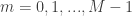
The first step in the analysis is to enumerate all possible sequences for the last three non-out events, along with their left-on-base and runs values. For a given number of PA, $M$ , there are $k^M$ distinct possible sequences. So the total we need to track is

$\Sigma_0^3 ~k^M = 5^0 + 5^1 + 5^2 +5^3 = 1 + 5 + 25 + 125 = 156$ .

As a couple examples,if the last three non-out PAs comprise 1 HR and 2 BB, then there are 3 sequences,

HR – BB – BB (1 run)
BB – HR – BB (2 runs)
BB – BB – HR (3 runs)

The full list of the 156 last-three non-out PA sequences is given as a CSV file here [1].

The next step is to account for the cases with more than 6 total (3 non-out) PA. As mentioned above, it’s only the last three PA that specify the number of left-on-base. Here we want to enumerate the combinations of events (prior to the last 3), since each permutation will lead to the same number of runs (as long as the last three non-out events are the same). We then join each such combination with the 125 last-three-sequences.

For any given number, $M$ , of non-out events, the number of distinct combinations is ${M + k - 1 \choose k - 1}$ . Here $k = 5$ , and I denote a combination with $n_0$ base-on-balls, $n_1$ singles, $n_2$ doubles, $n_3$ triples, and $n_4$ home runs as $(n_0, n_1, n_2, n_3, n_4)$ . Then, for any combination, the multiplicity, i.e. the number of permutations that correspond to distinct sequences, is $M! / (n_0! n_1! n_2! n_3! n_4!) = M! / \Pi n_i!$ .

As a concrete example, for 8 total PA, there are 5 non-out PA. For two of those five, we need to generate the possible sequences, and join them with the 125 distinct last-three sequences. There are ${2 + 5 -1 \choose 5 - 1} = 15$ possible combinations, enumerated below. Note that the sum of the multiplicities equals the total number of sequences, $k^M = 5^2 = 25$ .

combinations	multiplicity
(0, 0, 0, 0, 2)	1
(0, 0, 0, 1, 1)	2
(0, 0, 0, 2, 0)	1
(0, 0, 1, 0, 1)	2
(0, 0, 1, 1, 0)	2
(0, 0, 2, 0, 0)	1
(0, 1, 0, 0, 1)	2
(0, 1, 0, 1, 0)	2
(0, 1, 1, 0, 0)	2
(0, 2, 0, 0, 0)	1
(1, 0, 0, 0, 1)	2
(1, 0, 0, 1, 0)	2
(1, 0, 1, 0, 0)	2
(1, 1, 0, 0, 0)	2
(2, 0, 0, 0, 0)	1

To generate the different combinations, note that the they’re distinguished by the fact that there are $k$ slots, and the the sum of the slot values is $M$ . We can generate these combinations recursively, by starting with the solution for $M = 0$ , and noting that we can generate the solution for $M$ from the solutions for $m = 0, 1, ..., M-1$ , by adding $M - m$ to each solution in the set for $m$ , and removing duplicates. An example of this in Python is given in the CombinatricsInningSim github repo.

The final step in this combinatorical analysis is to specify probabilities for each of the possible non-out events and analyze the conditional distributions.

Probability distributions

The number of total PA, $N$ , has a negative binomial distribution so that the number of non-out event events $r$ is $r \sim {k + r - 1 \choose k} (1-p)^r p^k$ .

The distribution of combinations $P(C|N)$ , is multinomial, with a probability of

$(N! / \Pi n_i) ~\Pi p_i^{n_i}$

The distribution of sequences, given a combination, is uniform, and equal to the inverse of the multiplicity.

Probability distributions – example

To illustrate how this works, let’s start with a simple example that’s straight-forward to verify, and that doesn’t rely on assumptions about taking extra bases on hits, advancing bases on outs, etc. Specifically, let’s look at a model where the probability to draw a base on balls is 10%, to hit a HR 10%, and to make an out (not advancing any runners) 80%. It can be verified with a Markov chain approach (e.g. Tom Tango’s Javascript + HTML version, my Python version with arbitrary number of bases, my Markov chain API server) that the mean number of runs scored per inning is 0.45356. For the combinatorial approach, I can sum over the runs corresponding to a given PA and left on base pair, times the probability for that pair, i.e. $<R> = \Sigma R(N, L) \times P(N,L) = \Sigma R(N, L) P(S|C) P(C|N) P(N)$ . The probabilities for each run value (up to 17) are shown below, confirming the same 0.45356 result.

runs	prob	runs_contrib
0	7.014400e-01	0.000000e+00
1	1.909760e-01	1.909760e-01
2	7.364608e-02	1.472922e-01
3	2.409677e-02	7.229030e-02
4	7.148339e-03	2.859336e-02
5	1.986560e-03	9.932800e-03
6	5.269094e-04	3.161457e-03
7	1.349452e-04	9.446162e-04
8	3.363045e-05	2.690436e-04
9	8.200126e-06	7.380114e-05
10	1.963983e-06	1.963983e-05
11	4.634182e-07	5.097600e-06
12	1.079740e-07	1.295688e-06
13	2.488606e-08	3.235188e-07
14	5.682108e-09	7.954951e-08
15	1.283541e-09	1.925311e-08
16	2.853804e-10	4.566087e-09
17	5.737808e-11	9.754273e-10

Conditional distributions

One of the benefits of approaching the run scoring distribution with this combinatorics method is that we can straight-forwardly generate the conditional distributions of runs scored, e.g. R|N, R|C. The below shows the runs scored distributions, conditional on $N$ , for the same toy problem with BB and HR probabilities of 0.1. Note that for more than 6 total PA, the distribution for $N+1$ is the distribution for $N$ , but shifted over by one run. This is because, as far as run scoring, the only thing that matters is the sequence of the last 3 non-out PA – for any PA that happened before that, the player has been forced in, in one way or another (ignoring outs on the bases).

conditional_prob1 We could look at the same for any number of conditional variables, e.g. total number of bases, number of singles, wOBA, etc. For now I’ll leave this as an exercise for the reader and move on to the next topic.

Conditional variance

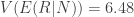
As illustrated above, the conditional value of a variable (e.g R|N, R|C) is itself a random variable. This means we can analyze the distribution, compute the mean, the variance, etc. The conditional variance [2] [3] is especially relevant for the current analysis.

In particular, if there are two random variables X and Y, there’s an identity regarding variance & conditional variance,

$V(Y) = V(E(Y|X)) + E(V(Y|X))$ ,

i.e., the variance of the random variable $Y$ can be decomposed into the variance left over after conditioning $Y$ on $X$ ( $E(V(Y|X))$ ), plus the variance due to the distribution of $X$ itself ( $V(E(Y|X))$ ).

In the run-scoring application, there are several different way to apply this.

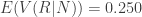
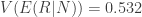
Conditional variance of runs given OBP

If we condition on total number of PA, $N$ , then we’re effectively isolating the variance at fixed OBP, which is due to both different linear-weights values and event sequencing. For the current example,with probability for HR = probability for BB = 10%, the variance breaks down as:

$E(V(R|N)) = 0.226$

$V(E(R|N)) = 0.464$

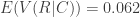
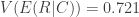
Conditional variance of runs given wOBA

On the other hand, if we condition on the combination of events, then we are very directly isolating the effect of sequencing. The results for the toy problem are:

$E(V(R|C)) = 0.0393$

$V(E(R|C)) = 0.6500$

Note that in both cases the total variance is the same, $V(R) = 0.6894$ .

More realistic numerical example

The above toy example is useful because it’s conceptually straight-forward. As a more realistic example I’ll set probabilities that roughly match historical MLB values, viz.:

BB: 0.08
1B: 0.15
2B: 0.05
3B: 0.005
HR: 0.025

Note that this corresponds to an OBP of 0.31. With these probabilities, the mean runs scored per inning is 0.353. This is lower than it would be in reality because I’m disregarding runners taking an extra base – this is the most substantive deficiency in the current analysis and will be addressed in a subsequent post.

With that said, here’s the breakdown of variance:

Conditional on $N$ (OBP)

$E(V(R|N)) = 0.250$

$V(E(R|N)) = 0.532$

Conditional on $C$ (linear-weights)

$E(V(R|C)) = 0.062$

$V(E(R|C)) = 0.721$

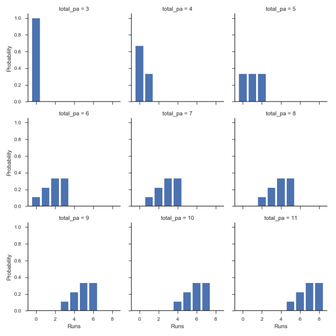
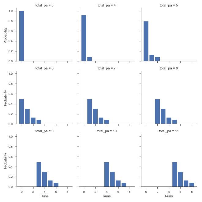
The conditional distribution of runs scored, for R|N is shown below

conditional_prob2

Empirical examples with retrosheet play-by-play data

We can apply these same principles of using the conditional distributions to isolate the different contributions to the overall variance of run scoring to empirical data. Here I use retrosheet play-by-play data to analyze runs scored conditional on $N$ and $C$ . For this analysis I’m using the data for 2006 through 2014.

First, the conditional distributions for $R|N$ ,

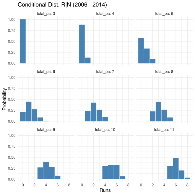
Note that for PA >= 6, the distribution does indeed have (mostly) the same shape, but is shifted over by one run for each extra PA, in agreement with the theoretical results from above.

The breakdown of variance for $R|N$ is,

$E(V(R|N)) = 0.238$

$V(E(R|N)) = 0.764$

and for $R|C$ ,

$E(V(R|C)) = 0.129$

$V(E(R|C)) = 0.876$

Runs for multiple innings

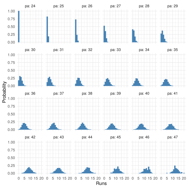
The results above focus on runs for a single inning. Here I look at a full game – or more specifically the first 8 innings of a game, in order to filter out the non-representative behavior (number of outs strategy, …) of the ninth inning. Analizing a full game is possible with the theoretical combinatorics approach also, but the number of combinations that need to be tracked gets unwieldy.

The below shows the conditional distribution of runs (first 8 innings) at given PA

The breakdown of variance for $R|N$ is,

$E(V(R|N)) = 2.68$

$V(E(R|N)) = 6.48$

and for $R|C$ ,

$E(V(R|C)) = 1.74$

$V(E(R|C)) = 7.62$

Conclusions

I’ve presented a theoretical / empirical way of analyzing the runs scored in a baseball game or inning using combinatorics. In an analysis of historical data provided by retrosheet, we find that the ratio of variance in run-scoring due to sequencing vs wOBA is $\sim 0.20$ , and of sequencing & linear weights vs OBP is $\sim 0.30$ .